Measuring & Optimizing I/O Performance
 Measuring and optimizing IO performance is somewhat of a black art: the tools are there, the resources and discussions are plenty, but it is also incredibly easy to get lost in the forest. I speak from recent experience. Having gone down multiple false starts with filesystem optimization, RAID tweaking, and even app-level changes it really helped to finally step back and revisit the basics. Many man pages and discussion threads later, a few useful realizations emerged: iostat is your best friend, but it can also be incredibly deceiving; refreshing your memory of disk latencies will go a long way; disks and filesystems are fast, but not that fast.
Monitoring IO Performance with iostat
If IO performance is suspect, iostat is your best friend. Having said that, the man pages are cryptic so don't be surprised if you find yourself reading the source. To get started, identify the device in question and start a monitoring process:
# -k output rates in kB
# -x output extended stats
# -d monitoring single device
# sample stats every 5 seconds for device /dev/sdh
$ iostat -dxk /dev/sdi 5
Next, allocate yourself a couple of hours to understand the output or expect to find yourself down a wrong path in no time flat (been there, done that). iostat is a popular tool amongst the database crowd, so not surprisingly you'll find a lot of great discussions documenting the use. Depending on your application you will need to focus on different metrics, but as a gentle introduction let's take a look at await, svctime and avgque:
- await - The average time (in milliseconds) for I/O requests issued to the device to be served. This includes the time spent by the requests in queue and the time spent servicing them.
- svctime - The average service time (in milliseconds) for I/O requests that were issued to the device.
- avgqu-sz - The average queue length of the requests that were issued to the device.

First off, await is a deceiving metric! Even though it claims to measure average time, it is better understood as an aggregate function, so don't be mislead by it: avgqu-sz * svctm / (%util/100). Ideally, await should be roughly equal to your svctime, which leads us to a corollary: your average queue size is ideally hovering around single digits. Understanding these variables alone can tell you volumes about the application generating the load.
Disk Latencies Refresher & EBS Performance
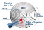
 Disk access time is determined via the sum of several variables: spin-up, seek, rotational delay, and transfer time. Assuming your disk is not is not sleeping we can discount the spin-up time, which leaves us with seek (time for the disk arm to find the track: ~10ms), rotational delay (time to get the right sector under the head: depends on RPM), and the actual transfer time. Hence, in the worst case we will take ~10ms to seek, 60s/7200RPM ~= 8ms in rotational delay, plus the read time. On average, for a 7.2k RPM disk this translates into roughly ~5ms access time (~20ms in worst case) to read the first byte!
Armed with this knowledge we can now put Amazon's EBS performance in context: on average our EBS mounts show 10~30ms svctime, which all things considered is not outrageous for a SAN. This number also dips into low single digits at nights and on weekends, which points to the fact that as with any shared resource, the performance of EBS degrades during the day. Having said that, a 6x performance difference based on time of day is definitely not anything to sneeze at, so let's hope Amazon is on top of this!
Average queue size (avgqu-sz) is a popular metric in the DBA circles, but do be careful with it when running on a SAN or any multi-spindle device. Ideally, your queue size (avgqu-sz) for a single disk should be in single digits, which means that the underlying device is well matched to the IO load generated by the application. Conversely, if the queue size is artificially low, chances are your application code can benefit from some tuning: do less disk flushing, think about caching or buffering, or in other words, double check the assumption that IO is the bottleneck!
Disks, Filesystems and Facebook Case Study: Haystack
 Average access time on our disks places some hard limits on the number of IOPs - at 5ms average, we get a very optimistic 200 req/s with no read time. Hence, if you're trying to store several hundred files a second, you might want to revisit the architecture or seriously think about switching to SSD's! Databases such as MySQL work around this constraint by minimizing the number of file handles, caching data, and using aggressive buffering techniques. Willing to potentially loose a little bit of data with InnoDB? Set flush_log_at_trx_commit to 2 to avoid flushing on every transaction in favor of a periodic one second flush. In similar fashion, you can tweak your MyISAM key buffers, or even place your index and data files on different drives.
Facebook team recently released the details of their Haystack photo storage system which serves as a great case study of working around the IO bottlenecks: over 15PB of photo storage, and ~360 new photos being uploaded every second as of April '09. To meet the requirements, they dropped the POSIX filesystem semantics and went for an append only structure with a separate in-memory index which stores the direct inode offsets for each photo. As a result, each photo access is translated into a single IO request - a huge win. Read through it, fascinating stuff and an illustrative example of optimizing for IO.
 Ilya Grigorik is a web ecosystem engineer, author of High Performance Browser Networking (O'Reilly), and Principal Engineer at Shopify — follow on Twitter.